Regression in terms of mathematics means a relationship between the values – particularly the output value with its corresponding values. Regression models in machine learning are used to predict real values. Let’s assume the case where we have a dataset that defines the salary trend in an organization on the basis of the experience of the employee in years. If the independent variable is experience, we can use the regression model to predict salary values of new employees entering the organization with different experience, or otherwise, our model can give us present but unknown salary values in the dataset.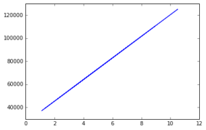

A simple linear regression refers to a straight sloped line with can mathematically be denoted with the equation :

y = mx+c

y = Dependent Variable. Its value is dependent upon the value of x.

x = Independent Variable.

m = Slope of the line

c = Constant

Click here to download the dataset along with the code.

For our dataset, the simple linear equation is as below:

Salary = m * Experience + c

The value of the constant c defines the basic salary of a fresher in the organization with 0 years of experience.

Ordinary Least Squares Method

The ordinary least squares method, also called as the Best Fitting line is another method used for simple linear regression. For this technique, the difference between the salary as per the model line(y = mx+c) is taken and stored. Assume that at some point, the salary is $50000, however as per the model it should be $48500. So the difference between the two i.e y2 – y1 is taken and is then squared i.e (y2 – y1)^2. For all the available data, such points are calculated and stored and the minimum value of the square values is selected. This line having the minimum (y2-y1)^2 will be called as the best-fitting line.

To create a machine learning algorithm that follows the simple linear regression approach, the first step is to preprocess the data. We will use the preprocessing template we already have. Once we load the dataset, we will use it to train our model using simple linear regression. As our model is trained, it will be able to understand the correlation between experience and salary and will be able to predict salary values for a given experience value. We will edit the data preprocessing template according to our dataset and once this is done, we will have the matrix of features- X and the dependent variable vector – Y along with their respective train and test sets.

The very basic step of the regression technique is to create a regressor. A regressor is an object of the regression class. This regressor is now a machine which is learning by getting experiences/observances from the training sets. The regressor understands the correlation between the salary and the experience. Comparing it to machine learning, the machine is the simple linear regressor model and learning is that the simple linear regressor machine learns from the training sets composed of X and Y variables – independent and dependent variables respectively.

#Fitting single linear regression to the Training Set
from sklearn.linear_model import LinearRegression
regressor = LinearRegression()
regressor.fit(X_train,y_train)

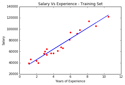
For finding out predictions, we create a vector called as y_pred to hold the prediction results. y_pred will be the vector of predictions of the dependent variable. We use the predict method of the regressor object to obtain the predictions for the test set. And finally, we use the matplotlib library to get a graphical representation of the salary predictions and the experience component.

#Predecting the Test set results
y_pred = regressor.predict(X_test)
y_train_pred = regressor.predict(X_train)
 
#Visualizing the Training set results
plt.scatter(X_train, y_train, color = 'red') #scatter graph
plt.plot(X_train,y_train_pred,color = 'blue') #regression line

See the complete python code for the case of simple linear regression technique for machine learning below :

# Data Preprocessing Template
 
# Importing the libraries
import numpy as np
import matplotlib.pyplot as plt
import pandas as pd
 
# Importing the dataset
dataset = pd.read_csv('Salary_Data.csv')
X = dataset.iloc[:, :-1].values
y = dataset.iloc[:, 1].values
 
# Splitting the dataset into the Training set and Test set
from sklearn.cross_validation import train_test_split
X_train, X_test, y_train, y_test = train_test_split(X, y, test_size = 1/3, random_state = 0)
#Fitting single linear regression to the Training Set
from sklearn.linear_model import LinearRegression
regressor = LinearRegression()
regressor.fit(X_train,y_train)
 
#Predecting the Test set results
y_pred = regressor.predict(X_test)
y_train_pred = regressor.predict(X_train)
 
#Visualizing the Training set results
plt.scatter(X_train, y_train, color = 'red') #scatter graph
plt.plot(X_train,y_train_pred,color = 'blue') #regression line
 
#labelling the plot
plt.title('Salary Vs Experience - Training Set')
plt.xlabel('Years of Experience')
plt.ylabel('Salary')
plt.show() #to mark the end of graph
 
 
#for test set
plt.scatter(X_test, y_test, color = 'red') #scatter graph
plt.plot(X_train,y_train_pred,color = 'blue') #regression line
 
#labelling the plot
plt.title('Salary Vs Experience - Test Set')
plt.xlabel('Years of Experience')
plt.ylabel('Salary')
plt.show() #to mark the end of graph